Markov Decision Process (MDP)#

How can we deal with uncertainty?

• A sequential decision problem for a fully observable, stochastic environment with Markovian transition and additive rewards.

Formal definition#

• MDP $M ≜ (S, A, T, R, γ)$
  • states $S$
  • actions $A$
  • Transition function $T$: $S, A, S' \rightarrow [0, 1]$
    • satisfies the Markov property s.t $\sum_{s'} T(s,a,s') = \sum_{s} P(s'|s,a) = 1$. (Sums to 1)
  • Reward function $R$
  • discount facrot $0 ≤ γ ≤ 1$
  • solution is a policy: a function that recommend an action in each state
• Markov property: Next state only determined by current state & action
  • $P(s_{t+1}|s_t, a_t, s_{t-1}, a_{t-1}, ..., s_0, a_0) = P(s_{t+1}|s_t, a_t)$
  • Markov property simplifies real-world problems
• Reward funciton $R(s,a,s')$: need to balance between risk & reward
• Policy $π: S \rightarrow A$: for every state, map an action
  • Quality of $π$: expected utility of sequence guaranteed by performing policy $π$
  • Optimal policy $π^*$: highest expected utility

Finite horizon:#

• fixed time $N$, then terminate
• Reward: sums up to $R_n$
• optimal action may change over time $\Rightarrow$ Nonstationary $π^*$

Infinite horizon:#

• no fixed deadline, may run forever
• Stationary $π^*$
• But R may be infinite, hard to compare policies.
  1. use discount factor $γ < 1$, utility becomes finite
     • $U_h([S_0, a_0, s_1, a_1,s_2, ...]) ≤ \frac {R_{max}} {1-γ}$
  2. Environment has terminal states, and policy guaranteed to get to a terminal state.
  3. Compute average rewards obtained per time stop
     • hard to compute and analyze

Utility of States#

• reward of executing $π^*(s)$
• Bellman Equation: $U(s) = U^{π^*}(s) = max_{a} \sum_{s'} P(s'|s,a)[R(s,a,s') + γU(s')] = V(s)$
• Optimal policy $π^*$ is the policy that maximizes $U(s)$: $π^*(s) = argmax_{a} \sum_{s'} P(s'|s,a)[R(s,a,s') + γU(s')]$
• Q-Function $Q(s,a)$: expected utility of taking a given action in a given state
  • $U(s) = max_a Q(s,a)$

Value Iteration#

• repeatedly perform Bellman Update
  • $U_{i+1}(s) ← max_a \sum_{s'} P(s'|s,a) [R(s,a,s') + \gamma U_i(s')]$ or
  • $U_{i+1}(s) \leftarrow R(s) + \gamma max_{a \in A(s)} \sum_{s'} P(s'|s,a) U_i(s')$
• to find rewarding value for each state
• initialize as $0$, iterate until convergence

Policy Iteration#

• Begin with initial policy $π_0$
• Repeat until no change in Utility for each state:
  1. Policy evaluation: uses the given policy to calculate the utility of each state
  2. Policy improvement:
     • find the best action for $π_i$ via one-step lookahead based on $U_i$ obtained from policy evaluation step
     • $π_{i+1}(s) = argmax_a \sum_{s'} P(s'|s,a)[R(s,a,s') + γU_{π_k}(s')]$
• Complexity: $S = n$ linear equations with $n$ unknowns $\Rightarrow$ $O(n^3)$
• Policy iteration may be faster than value iteration.

Online Algorithms#

Decision-time planning

• for large problems, state space increase exponentially
• we can use Online search with sampling
  • real time dynamic programming
  • Monte Carlo Tree Search
• 
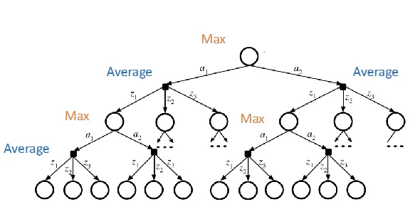
• keep the best actions at each state nodes
• tree size: $A^D S^D$, A is the # of actions, S is the # of states, D is the depth of tree
• With sparse sampling:
  • sampling $k$ observations
  • tree size: $A^D k^D$
  • but still exponential with search depth

Monte Carlo Tree Search#

Online search with simulation

• 
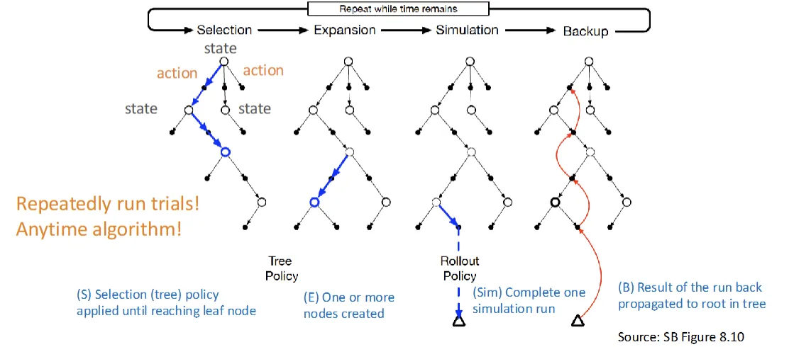
• Selection: select the leave nodes to expand
  • Selection policy: Upper Confidence Bounds applied to Trees(UCT)
    • $π_{UCT}(n) = argmax_{a}(\hat{Q}(n,a) + c \sqrt{\frac {N(n)}{N(n,a)}}$
      • $\hat{q}(n,a)$ is the average return of all trials (exploitation)
      • $c$: constant balancing exploitation & exploration
      • $N(n)$: # of trials through node $n$
      • $N(n,a)$: # of trials through node $n$ starting with $a$
    • 也等於 $π_{UCT}(n) = \frac {U(n)}{N(n)} + C \sqrt{\frac {log N(Parent(n))}{N(n)}}$
      • $N(Parent(n))$: the # of parent node been visited
      • $N(n)$: the # of node $n$ been visited.
      • $\frac {U(n)}{N(n)}$: 贏的次數 / 嘗試的次數
      • $\sqrt{\frac {log N(Parent(n))}{N(n)}}$: 開根號 $log$總次數 / 嘗試的次數
• Expansion: one or more nodes created
• Simulation: estimate the value of the node by completing one simulation run (run to leaf)
• Backup: update the result back to root.