Motivation#

intractable integration problems

• Normalization: $p(x|y) = \frac {p(y|x)p(x)}{\int_x p(y|x')p(x')dx'}$
  • $\int_x p(y|x')p(x')dx'$ is intractable to compute in high dimension
• Marinalization: $p(x|y) = \int_z p(x, z|y)dz$
• Expectation: $E_{p(x|y)}[f(x)] = \int_x f(x)p(x|y)dx$

Weak law of large numbers#

• $\bar x_n \xrightarrow p \mu$ when $n \rightarrow \infty$
  • $\bar x_n$: sample average $= \frac {1}{n} \sum_n x_n$
  • $\mu$: real average $= \int x p(x) dx$

Strong law of large numbers#

• $\bar x_n \xrightarrow {a.s \ (converges)} \mu$ when $n \rightarrow \infty$
  • $\bar x_n$: sample average $= \frac {1}{n} \sum_n x_n$
  • $\mu$: real average $= \int x p(x) dx$

Non parametric representation#

• represent with drawing samples
• the higher probability of an interval, the more samples are drawn in the intervalf

Rejection Sampling#

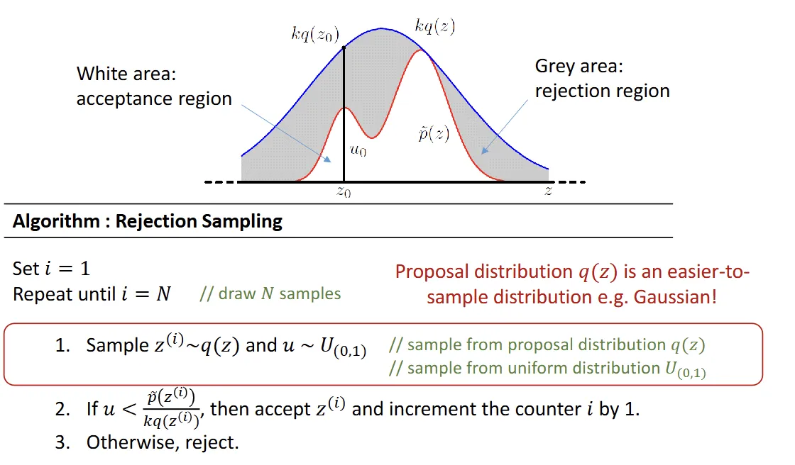
• $\tilde p(z)$: target
• $\tilde q(z)$: proposal
• set $k$ so that $k \tilde q(z) \geq \tilde p(z)$

Limitation#

• not always possible for $k$ to cover all $\tilde p(z)$
• if $k$ too large, probability of $z$ is accepted $= Pr(u < \frac {\tilde p(z)}{k \tilde q(z)}) = \frac {1}{k}$

Importance Sampling#

• approximating expectations of a function $f(z)$ w.r.t $p(z)$ (target) samples from $q(z)$ (proposal)
• $E[f] = \int f(z)p(z) dz = \int f(z) \frac {p(z)}{q(z)} q(z) dz \approx \frac {1}{L} \sum{L} \frac {q(z^l)}{p(z^l)} f(z^l)$
• therefore importance weight $r_l = \frac {p(z^l)}{q(z^l)}$
• but $p(z^l)$ is hard to get , $\tilde p(z^l)$ is easy to get (unnormalized)
• $\Rightarrow E[f] = \frac {Z_q}{Z_p} \frac {1}{L} \sum_l^L \tilde r_l f(z^l)$, $\tilde r_l = \frac {\tilde p(z^l)}{\tilde q(z^l)}$
• $Rightarrow E[f] = \sum_l^L w_l f(z^l)$, $w_l = \frac {\frac {\tilde p(z^l)}{q(z^l)}}{\sum_m \frac {p(z^m)}{q(z^m)}}$

Limitation#

• not able to cover everything in the target distribution
• weight may be dominated by a few having large numbers

Ancestral Sampling#

• all weights $=1$
• starts with root nodes (easy to sample)
• troublesome if loop $\rightarrow$ randomly initialize, but may not converge

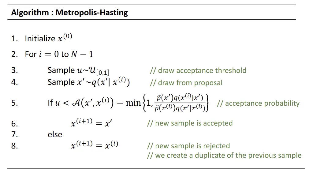
MCMC#

• spend more time in the most important regions.
• use adaptive proposals: use $q(x'|x)$ instead of $q(x')$
  • $x$: the previous sample
  • $x'$: the new sample
• 

Burn-In period#

• initial samples may be useles
• discard the first few samples (e.g 1000)

Markov Chain properties#

1. Homogeneous: fixed transition matrix
2. Stationary & limiting distribution: $\pi T = \pi$ (will eventually converge)
3. Irreducibility: at any state, there’s a probability $>0$ to visit all other states (will not get stuck at a state)
4. Aperiodicity: won’t get trapped in a cycle
5. Ergodic: Irreducibility + Aperiodicity. MCMC algorithms must satisfy ergodic
6. Detailed balance (Reversibility): $\pi_a T_{ab} = \pi_b T_{ba}$

• Metropolis-Hasting works because it satisfies detailed balance

Metropolis Algorithm#

• a special case of the Metropolis-Hasting
• random walk
• acceptance probability $AA(x',x) = min \{1, \frac {\tilde p(x')}{\tilde p(x)} \}$

Gibbs Sampling#

• a special case of the Metropolis-Hasting
• acceptance probability is always 1
• 
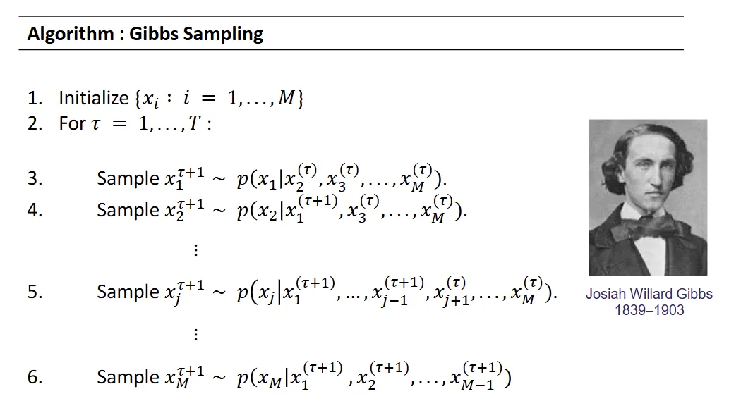
• condition on all other nodes
• use Markov Blanket (parents, childrens & co-parents) or $1^{st}$ degree neighbor for MRF

After we have samples:#

• $P(B)$: count # of $B=0$ and $B=1$
• becomes statistic