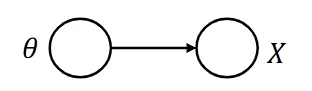
Goal: How to get unknown parameter θ \theta θ p ( x 1 , . . . , x M ∣ θ ) p(x_1, ..., x_M | \theta) p ( x 1 , ... , x M ∣ θ ) fully observed data (x 1 , . . . , x M x_1, ... ,x_M x 1 , ... , x M
Given: a set of N N N independent and identically distributed (i.i.d) complete observation of each random variable X : { x 1 , 1 , . . . x 1 , N , . . . x M , 1 , . . . , x M , N } X: \{ x_{1,1}, ... x_{1,N}, ...x_{M,1}, ..., x_{M,N}\} X : { x 1 , 1 , ... x 1 , N , ... x M , 1 , ... , x M , N }
M M M N N N Method:
Maximum likelihood estimate (MLE) Maximum a posteriori (MAP) Maximum Likelihood Estimate (MLE)# find the unknown parameters θ \theta θ likelihood p ( x 1 , . . . , x M ∣ θ ) p(x_1, ..., x_M| \theta) p ( x 1 , ... , x M ∣ θ )
θ ^ = a r g m a x θ [ p ( x 1 , . . . , x M ∣ θ ) ] \hat \theta = argmax_\theta [p(x_1, ..., x_M| \theta)] θ ^ = a r g ma x θ [ p ( x 1 , ... , x M ∣ θ )] = a r g m a x θ [ ∏ i = 1 N p ( x 1 , i , . . . x M , i ∣ θ ) ] = argmax_\theta [\prod_{i=1}^N p(x_{1,i}, ... x_{M,i} | \theta)] = a r g ma x θ [ ∏ i = 1 N p ( x 1 , i , ... x M , i ∣ θ )] ∏ i = 1 N p ( x 1 , i , . . . x M , i ∣ θ ) = p ( x 1 , 1 , . . . x M , 1 ∣ θ ) × p ( x 1 , 2 , . . . x M , 2 ∣ θ ) × . . . × p ( x 1 , N , . . . x M , N ∣ θ ) \prod_{i=1}^N p(x_{1,i}, ... x_{M,i} | \theta) = p(x_{1,1}, ... x_{M,1} | \theta) \times p(x_{1,2}, ... x_{M,2} | \theta) \times ... \times p(x_{1,N}, ... x_{M,N} | \theta) ∏ i = 1 N p ( x 1 , i , ... x M , i ∣ θ ) = p ( x 1 , 1 , ... x M , 1 ∣ θ ) × p ( x 1 , 2 , ... x M , 2 ∣ θ ) × ... × p ( x 1 , N , ... x M , N ∣ θ ) Maximum a Posteriori (MAP)# find the unknown parameters θ \theta θ a posterior probability p ( θ ∣ x 1 , . . . , x M ) p(\theta | x_1, ..., x_M) p ( θ ∣ x 1 , ... , x M )
θ ^ = a r g m a x θ [ p ( θ ∣ x 1 , . . . x M ) ] = a r g m a x θ [ p ( x 1 , . . . x M ∣ θ ) p ( θ ) p ( x 1 , . . . x M ) ] \hat \theta = argmax_\theta [p(\theta | x_1, ... x_M)] \\ = argmax_\theta [\frac {p(x_1, ...x_M| \theta)p(\theta)}{p(x_1, ...x_M)}] θ ^ = a r g ma x θ [ p ( θ ∣ x 1 , ... x M )] = a r g ma x θ [ p ( x 1 , ... x M ) p ( x 1 , ... x M ∣ θ ) p ( θ ) ] = a r g m a x θ [ ∏ i = 1 N p ( x 1 , i , . . . , x m , i ∣ θ ) [ ( θ ) ] p ( x 1 , . . . , x M ) ] = argmax_\theta [\frac {\prod_{i=1}^N p(x_{1,i}, ..., x_{m,i} | \theta) [(\theta)]}{\cancel{p(x_1, ..., x_M)}}] = a r g ma x θ [ p ( x 1 , ... , x M ) ∏ i = 1 N p ( x 1 , i , ... , x m , i ∣ θ ) [( θ )] ] p ( x 1 , . . . , x M ) p(x_1, ..., x_M) p ( x 1 , ... , x M ) θ \theta θ = a r g m a x θ [ ∏ i = 1 N p ( x 1 , i , . . . , x M , i ∣ θ ) p ( θ ) ] ] = argmax_\theta [\prod_{i=1}^N p(x_{1,i}, ..., x_{M,i} | \theta)p(\theta)]] = a r g ma x θ [ ∏ i = 1 N p ( x 1 , i , ... , x M , i ∣ θ ) p ( θ )]] Example: Single Random Variable DGM#
Continuous DGM# Univariate Normal Distribution
p ( x ∣ θ ) = N o r m x [ μ , σ 2 ] = 1 2 π σ 2 e − ( x − μ ) 2 2 σ 2 p(x|\theta) = Norm_x [\mu, \sigma^2] = \frac{1}{\sqrt {2 \pi \sigma^2}} e^{- \frac {(x-\mu)^2}{2 \sigma^2}} p ( x ∣ θ ) = N or m x [ μ , σ 2 ] = 2 π σ 2 1 e − 2 σ 2 ( x − μ ) 2 goal is to find the two unknown parameters θ = ( μ , σ 2 ) \theta = (\mu, \sigma^2) θ = ( μ , σ 2 ) M1: Maximum Likelihood Estimation (MLE)
θ ^ = a r g m a x θ [ p ( x t h e t a ) ] = a r g m a x θ [ ∏ i = 1 N p ( x [ i ] ∣ θ ) ] \hat \theta = argmax_\theta [p(x\ theta)] \\ = argmax_\theta [\prod_{i=1}^N p(x[i] | \theta)] θ ^ = a r g ma x θ [ p ( x t h e t a )] = a r g ma x θ [ ∏ i = 1 N p ( x [ i ] ∣ θ )] p ( x ∣ θ ) = p ( x ∣ μ , σ 2 ) = ∏ i = 1 N N o r m x [ i ] [ μ , σ 2 ] p(x| \theta) = p(x| \mu, \sigma^2) = \prod_{i=1}^N Norm_{x[i]} [\mu, \sigma^2] p ( x ∣ θ ) = p ( x ∣ μ , σ 2 ) = ∏ i = 1 N N or m x [ i ] [ μ , σ 2 ] maximize the logarithm μ ^ , σ ^ 2 = a r g m a x μ , σ 2 ∑ i = 1 N l o g [ N o r m x [ i ] [ μ , σ 2 ] ] = a r g m a x μ , σ 2 [ − 0.5 N l o g [ 2 π ] − 0.5 N l o g σ 2 − 0.5 ∑ i = 1 N ( x [ i ] − μ ) 2 σ 2 ] \hat \mu, \hat \sigma^2 = argmax_{\mu, \sigma^2} \sum_{i=1}^N log[Norm_{x[i]}[\mu, \sigma^2]] \\ = argmax_{\mu, \sigma^2}[-0.5N log[2\pi] - 0.5Nlog \sigma^2 - 0.5\sum_{i=1}^N \frac {(x[i]-\mu)^2}{\sigma^2}] μ ^ , σ ^ 2 = a r g ma x μ , σ 2 ∑ i = 1 N l o g [ N or m x [ i ] [ μ , σ 2 ]] = a r g ma x μ , σ 2 [ − 0.5 Nl o g [ 2 π ] − 0.5 Nl o g σ 2 − 0.5 ∑ i = 1 N σ 2 ( x [ i ] − μ ) 2 ] ∂ L ∂ μ = ∑ i = 1 N ( x [ i ] − μ ) 2 σ 2 = ∑ i = 1 N x [ i ] σ 2 − N μ σ 2 = 0 \frac {\partial L}{\partial \mu} = \sum_{i=1}^N \frac {(x[i]-\mu)^2}{\sigma^2} = \frac{\sum_{i=1}^N x[i]}{\sigma^2} - \frac {N \mu}{\sigma^2}= 0 ∂ μ ∂ L = ∑ i = 1 N σ 2 ( x [ i ] − μ ) 2 = σ 2 ∑ i = 1 N x [ i ] − σ 2 N μ = 0 0 0 0 ∂ L ∂ σ 2 = − N σ 2 + ∑ i = 1 N ( x [ i ] − μ ) 2 σ 4 = 0 \frac {\partial L}{\partial \sigma^2} = - \frac{N}{\sigma^2} + \sum_{i=1}^N \frac{(x[i]-\mu)^2}{\sigma^4} = 0 ∂ σ 2 ∂ L = − σ 2 N + ∑ i = 1 N σ 4 ( x [ i ] − μ ) 2 = 0 we get μ ^ = ∑ i = 1 N x [ i ] N = x ˉ \hat \mu = \frac {\sum_{i=1}^N x[i]}{N} = \bar x μ ^ = N ∑ i = 1 N x [ i ] = x ˉ σ ^ 2 = ∑ i = 1 N ( x [ i ] − μ ) 2 N \hat \sigma^2 = \frac {\sum_{i=1}^N (x[i] - \mu)^2}{N} σ ^ 2 = N ∑ i = 1 N ( x [ i ] − μ ) 2 Maximum likelihood for the normal distribution gives least squares fittingμ ^ = a r g m a x μ − ∑ i = 1 N ( x [ i ] − μ ) 2 = a r g m i n μ ∑ i = 1 N ( x [ i ] − μ ) 2 \hat \mu = argmax_\mu -\sum_{i=1}^N (x[i] - \mu)^2 = argmin_\mu \sum_{i=1}^N (x[i] - \mu)^2 μ ^ = a r g ma x μ − ∑ i = 1 N ( x [ i ] − μ ) 2 = a r g mi n μ ∑ i = 1 N ( x [ i ] − μ ) 2 M2: Maximum a Posteriori (MAP)
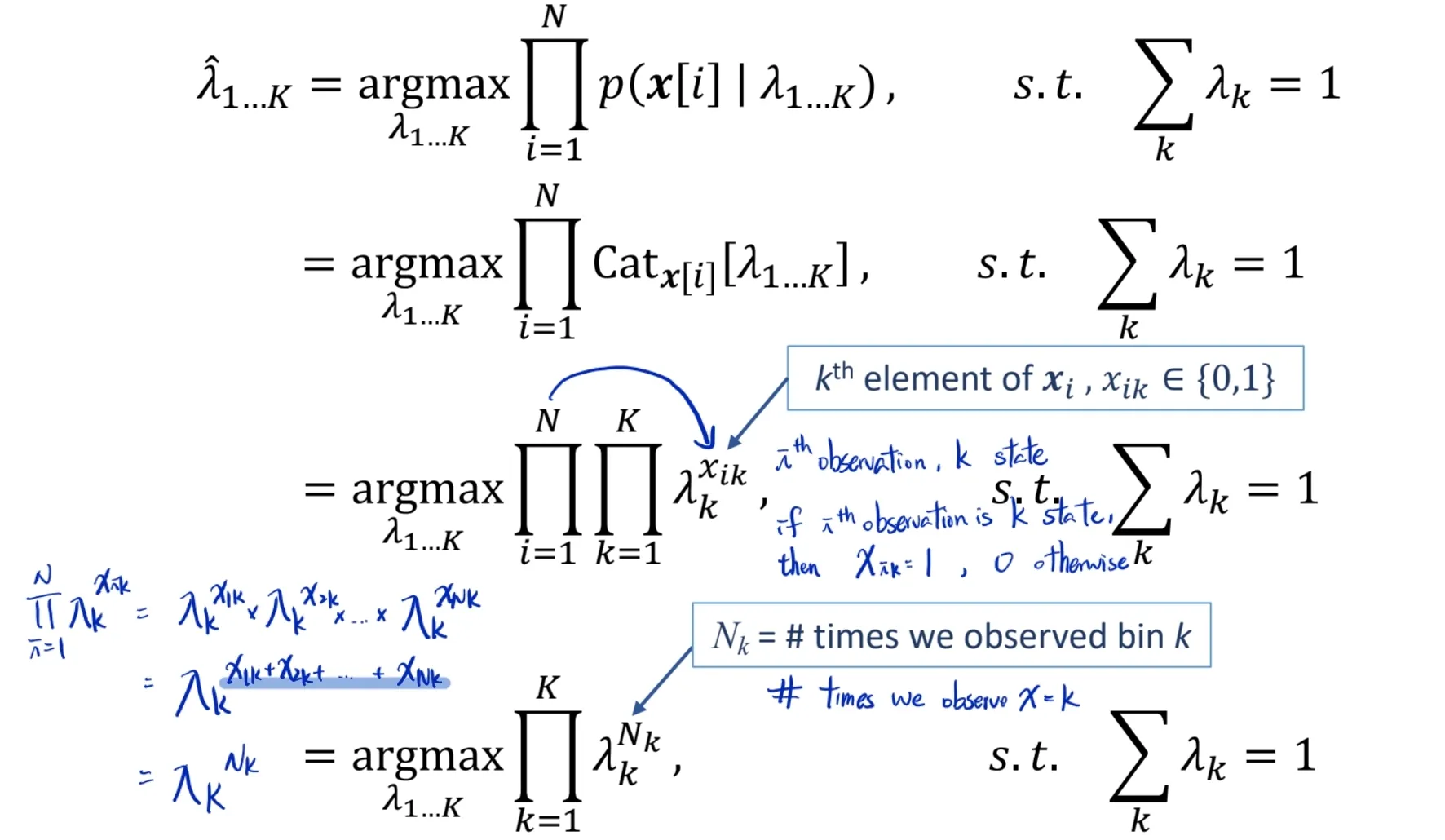
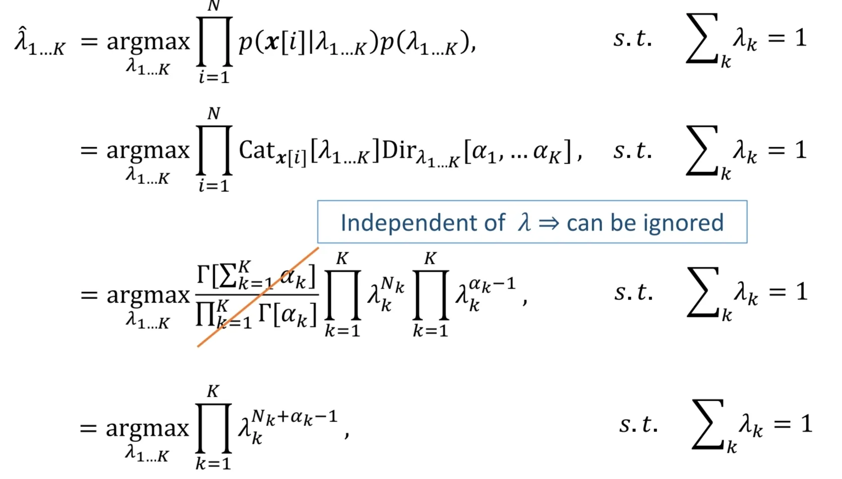
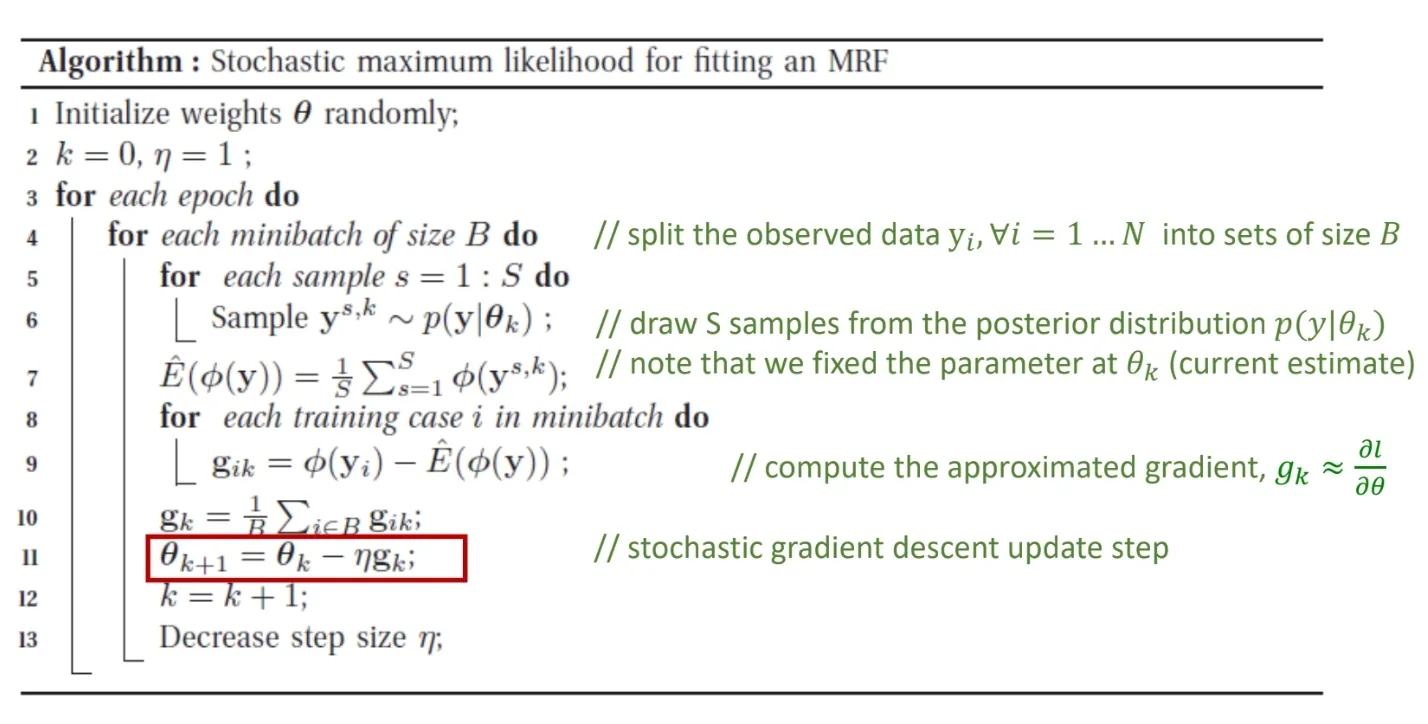
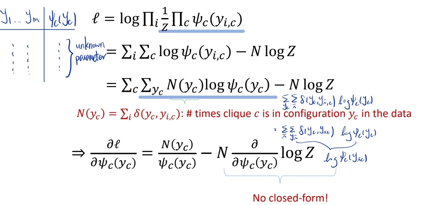
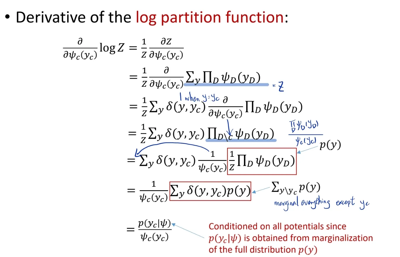
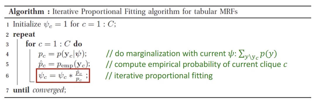
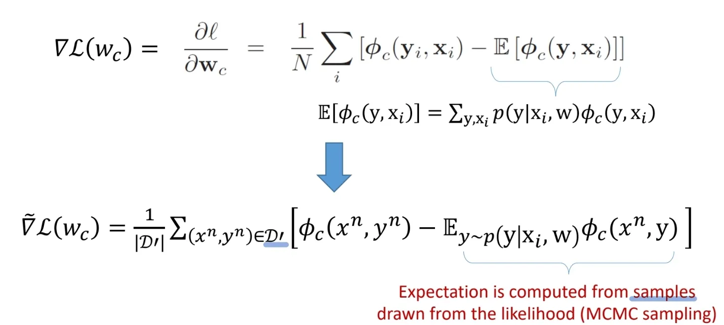
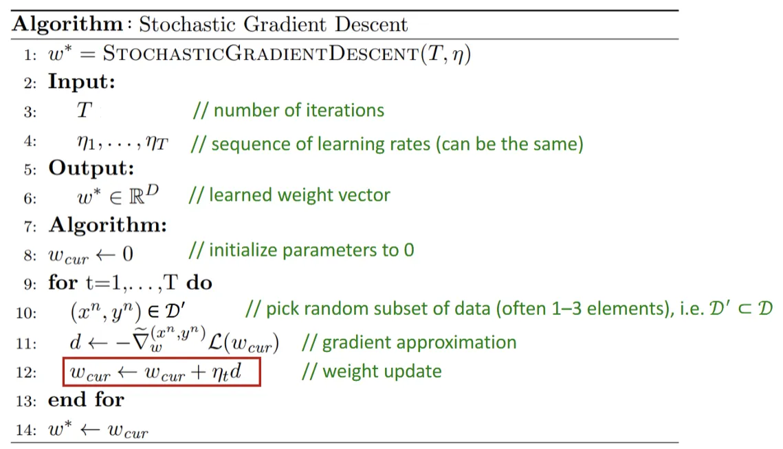
θ ^ = a r g m a x θ [ ∏ i = 1 N p ( x [ i ] ∣ θ ) p ( θ ) ] \hat \theta = argmax_\theta [\prod_{i=1}^N p(x[i]|\theta)p(\theta)] θ ^ = a r g ma x θ [ ∏ i = 1 N p ( x [ i ] ∣ θ ) p ( θ )] p ( x [ i ] ∣ θ ) p(x[i]|\theta) p ( x [ i ] ∣ θ ) p ( x ∣ μ , σ 2 ) = ∏ i = 1 N N o r m x [ i ] [ μ , σ 2 ] p(x|\mu, \sigma^2) = \prod_{i=1}^N Norm_{x[i]} [\mu, \sigma^2] p ( x ∣ μ , σ 2 ) = ∏ i = 1 N N or m x [ i ] [ μ , σ 2 ] p ( θ ) p(\theta) p ( θ ) p ( μ , s i g m a 2 ) = N o r m I n v G a m μ , σ 2 [ α , β , γ , δ ] p(\mu, sigma^2) = NormInvGam_{\mu, \sigma^2}[\alpha, \beta, \gamma, \delta] p ( μ , s i g m a 2 ) = N or m I n v G a m μ , σ 2 [ α , β , γ , δ ] μ ^ , σ ^ 2 = a r g m a x μ , σ 2 [ ∏ i = 1 N N o r m x [ i ] [ μ , σ 2 ] N o r m I n v G a m μ , σ 2 [ α , β , γ , δ ] ] \hat \mu, \hat \sigma^2 = argmax_{\mu, \sigma^2} [\prod_{i=1}^N Norm_{x[i]} [\mu, \sigma^2] NormInvGam_{\mu, \sigma^2}[\alpha, \beta, \gamma, \delta]] μ ^ , σ ^ 2 = a r g ma x μ , σ 2 [ ∏ i = 1 N N or m x [ i ] [ μ , σ 2 ] N or m I n v G a m μ , σ 2 [ α , β , γ , δ ]] Maximize the logarithmμ ^ , σ ^ 2 = a r g m a x μ , σ 2 [ ∑ i = 1 N l o g [ N o r m x [ i ] [ μ , σ 2 ] ] + l o g [ N o r m I n v G a m μ , σ 2 [ α , β , γ , δ ] ] \hat \mu, \hat \sigma^2 = argmax_{\mu, \sigma^2} [\sum_{i=1}^N log [Norm_{x[i]} [\mu, \sigma^2]] + log[ NormInvGam_{\mu, \sigma^2}[\alpha, \beta, \gamma, \delta]] μ ^ , σ ^ 2 = a r g ma x μ , σ 2 [ ∑ i = 1 N l o g [ N or m x [ i ] [ μ , σ 2 ]] + l o g [ N or m I n v G a m μ , σ 2 [ α , β , γ , δ ]] Take the derivatives of μ \mu μ σ 2 \sigma^2 σ 2 0 0 0 Discrete DGM# p ( X = e k ∣ θ ) = C a t x [ λ ] = ∏ k = 1 K λ k x k = λ k p(X=e_k|\theta) = Cat_x[\lambda] = \prod_{k=1}^K \lambda_k^{x_k} = \lambda_k p ( X = e k ∣ θ ) = C a t x [ λ ] = ∏ k = 1 K λ k x k = λ k k k k Goal: find the K K K θ = { λ 1 , . . . , λ K } \theta = \{ \lambda_1, ..., \lambda_K \} θ = { λ 1 , ... , λ K } λ k ∈ [ 0 , 1 ] \lambda_k \in [0,1] λ k ∈ [ 0 , 1 ] ∑ k λ k = 1 \sum_k \lambda_k = 1 ∑ k λ k = 1 M1: Maximum Likelihood Estimation (MLE) θ ^ = a r g m a x θ [ p ( x ∣ θ ) ] = a r g m a x θ [ ∏ i = 1 N p ( x [ i ] ∣ t h e t a ) ] \hat \theta = argmax_\theta [p(x|\theta)] = argmax_\theta[\prod_{i=1}^N p(x[i]|theta)] θ ^ = a r g ma x θ [ p ( x ∣ θ )] = a r g ma x θ [ ∏ i = 1 N p ( x [ i ] ∣ t h e t a )] p ( x l a m b d a ) = ∏ i = 1 N C a t x [ i ] [ λ 1... K ] = ∏ i = 1 N ∏ k = 1 K λ k x i k p(x\ lambda) = \prod_{i=1}^N Cat_{x[i]} [\lambda_{1...K}] = \prod_{i=1}^N \prod_{k=1}^K \lambda_k^{x_{ik}} p ( x l amb d a ) = ∏ i = 1 N C a t x [ i ] [ λ 1... K ] = ∏ i = 1 N ∏ k = 1 K λ k x ik apply the Lagrange multipier v v v L = ∑ k = 1 K N k l o g [ λ k ] + v ( ∑ k = 1 K λ k − 1 ) L = \sum_{k=1}^K N_k log[\lambda_k] + v (\sum_{k=1}^K \lambda_k-1) L = ∑ k = 1 K N k l o g [ λ k ] + v ( ∑ k = 1 K λ k − 1 ) take the derivative of L L L λ k \lambda_k λ k v v v 0 0 0 λ k \lambda_k λ k M2: Maximum a Posteriori (MAP) Likelihood [ ( x ∣ λ ) [(x|\lambda) [( x ∣ λ ) Prior: Dirichlet distributionp ( λ 1 , . . . , λ K ) = D i r λ 1... K [ α 1 , . . . α K ] p(\lambda_1, ..., \lambda_K) = Dir_{\lambda_{1...K}} [\alpha_1, ...\ \alpha_K] p ( λ 1 , ... , λ K ) = D i r λ 1... K [ α 1 , ... α K ] apply the Lagrange multiplier v v v L = ∑ k = 1 K ( N k + α k − 1 ) l o g λ k + v ( ∑ k = 1 K λ k − 1 ) L = \sum_{k=1}^K (N_k + \alpha_k -1) log \lambda_k + v (\sum_{k=1}^K \lambda_k -1) L = ∑ k = 1 K ( N k + α k − 1 ) l o g λ k + v ( ∑ k = 1 K λ k − 1 ) take the derivative of L L L λ k \lambda_k λ k v v v 0 0 0 λ k \lambda_k λ k Parameter Learning in UGM (MRF)# for example, a MRF in log-linear formp ( y ∣ θ ) = 1 Z ( θ ) e ∑ c θ c T ø c ( y ) p(y| \theta) = \frac{1}{Z(\theta)}e^{\sum_c \theta_c^T ø_c(y)} p ( y ∣ θ ) = Z ( θ ) 1 e ∑ c θ c T ø c ( y ) scaled log-likelihood: l ( θ ) = 1 N ∑ i N l o g p ( y i ∣ θ ) = 1 N ∑ i N [ ∑ c θ c T ø c ( y i ) − l o g Z ( θ ) ] l(\theta) = \frac{1}{N} \sum_i^N log p(y_i|\theta) = \frac {1}{N} \sum_i^N [\sum_c \theta_c^T ø_c(y_i) - log Z(\theta)] l ( θ ) = N 1 ∑ i N l o g p ( y i ∣ θ ) = N 1 ∑ i N [ ∑ c θ c T ø c ( y i ) − l o g Z ( θ )] Since MRFs are in the exponential family, this function is convex in θ \theta θ it has a unique global maximum, we can use the gradient-based optimizers the derivative of the log partition function w.r.t θ c \theta_c θ c c t h c^{th} c t h ∂ l o g Z ( θ ) ∂ θ c = E [ ø c ( y ) ∣ θ ] = ∑ y ø c ( y ) p ( y ∣ θ ) \frac {\partial log Z(\theta)}{\partial \theta_c} = E[ø_c(y)|\theta] = \sum_y ø_c(y) p(y|\theta) ∂ θ c ∂ l o g Z ( θ ) = E [ ø c ( y ) ∣ θ ] = ∑ y ø c ( y ) p ( y ∣ θ ) gradient of the log-likelihood is ∂ l ∂ θ c = 1 N ∑ i N ø c ( y i ) − E [ ø c ( y ) ] = 0 \frac {\partial l}{\partial \theta_c} = \frac{1}{N} \sum_i^N ø_c(y_i) - E[ø_c(y)] = 0 ∂ θ c ∂ l = N 1 ∑ i N ø c ( y i ) − E [ ø c ( y )] = 0 = E p e m p [ ø c ( y ) ] − E p ( y ∣ θ ) [ ø c ( y ) ] = 0 = E_{p_{emp}} [ø_c(y)] - E_{p(y|\theta)}[ø_c(y)] = 0 = E p e m p [ ø c ( y )] − E p ( y ∣ θ ) [ ø c ( y )] = 0 Sol: use gradient-based optimizers + approximate inference M1: Stochastic Maximum Likelihood stochastic gradient descent method iteratively update the parmeter θ k + 1 \theta_{k+1} θ k + 1 k k k θ k + 1 ← θ k − η g k \theta_{k+1} \leftarrow \theta_k - \eta g_k θ k + 1 ← θ k − η g k M2: Iterative Proportional Fitting (IFP) alternative derivation of the gradient in term of ψ c ( y c ) \psi_c(y_c) ψ c ( y c ) Parameter learning in UGM (CRF)# scaled log-likelihood: l ( w ) = 1 N ∑ i N l o g p ( y i ∣ x i , w ) = 1 N ∑ i N [ ∑ c w c T ø c ( y i , x i ) − l o g Z ( w , x i ) ] l(w) = \frac{1}{N} \sum_i^N log p(y_i|x_i,w) = \frac{1}{N} \sum_i^N [\sum_c w_c^T ø_c(y_i,x_i) - log Z(w,x_i)] l ( w ) = N 1 ∑ i N l o g p ( y i ∣ x i , w ) = N 1 ∑ i N [ ∑ c w c T ø c ( y i , x i ) − l o g Z ( w , x i )] gradients: ∂ l ∂ w c = 1 N ∑ i N [ ø c ( y i , x i ) − E [ ø c ( y , x i ) ] ] \frac {\partial l}{\partial w_c} = \frac {1} {N} \sum_i^N [ø_c(y_i, x_i) - E[ø_c(y, x_i)]] ∂ w c ∂ l = N 1 ∑ i N [ ø c ( y i , x i ) − E [ ø c ( y , x i )]] approximate the gradient with MCMC samples we can also do a MAP estimation of the unknown parameter in CRFa r g m a x w [ ∑ i l o g p ( y i ∣ x i , w ) + l o g p ( w ) ] argmax_w[\sum_i log p(y_i|x_i, w) + log p(w)] a r g ma x w [ ∑ i l o g p ( y i ∣ x i , w ) + l o g p ( w )] Gaussian prior is often userd for p ( w ) p(w) p ( w )