Goal: To calculate $p(x_F|x_E)$

• where $x_F$, $x_E$ are disjoint subsets
• $x_F$: query node
  $x_E$: evidence node
• needs to marginalize all nuisance variables $x_R$ ($x_V - (x_E, x_F)$)
  • $p(x_F | x_E) = \frac {p(x_F, x_E)} {p(x_E)} = \frac {\sum_{x_R} p(x_f, x_e, x_R)}{\sum_{x_F} p(x_F, x_E)} \Rightarrow O(K^n)$ (exponential, intractable!)

Variable elimination (the naive way)#

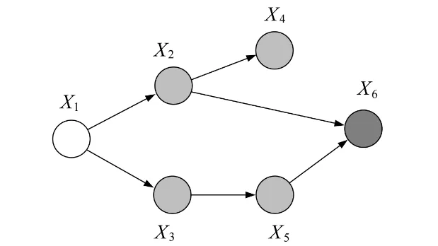
• $p(x_1, ..., x_5) = \sum_{x_6} p(x1)p(x_2|x_1)p(x_3|x_1)p(x_4|x_2)p(x_5|x_3)p(x_6|x_3, x_5) \\ = p(x1)p(x_2|x_1)p(x_3|x_1)p(x_4|x_2)p(x_5|x_3) \sum_{x_6} (x_6|x_3, x_5) \Rightarrow$ reduced table size to $K^3$
• When evidence node is observed ($x_6 = \bar x_6$):
  • e.g $p(x_6|x_2, x_5) \Rightarrow p(x_6 = 1 | x_2, x_5)$
    table from 3D ($x_2, x_5, x_6$) to 2D ($x_2, x_5$), $x_6=1$
  • $p(x_1|\bar x_6) = \sum_{x_2} \sum_{x_3} \sum_{x_4} \sum_{x_5} p(x_1)p(x_2|x_1)p(x_3|x_1)p(x_4|x_2)p(x_5|x_3)p(\bar x_6|x_3, x_5) \\ = p(x_1) \sum_{x_2} p(x_2|x_1) \sum_{x_3} p(x_3|x_1) \sum_{x_4} p(x_4|x_2) \sum_{x_5} p(x_5|x_3)p(\bar x_6|x_3, x_5) \\ = p(x_1) \sum_{x_2} p(x_2|x_1) \sum_{x_3} p(x_3|x_1) \sum_{x_4} p(x_4|x_2) \times m_5 (x_2, x_3) \\ = p(x_1) \sum_{x_2} p(x_2|x_1) \sum_{x_3} p(x_3|x_1) m_5 (x_2, x_3) \sum_{x_4} p(x_4|x_2) \\ = p(x_1) \sum_{x_2} p(x_2|x_1) m_4(x_2)\sum_{x_3} p(x_3|x_1) m_5 (x_2, x_3) \\ = p(x_1) \sum_{x_2} p(x_2|x_1) m_4(x_2) m_3(x_1, x_2) \\ = p(x_1) m_2(x_1) \\ = p(x_1, \bar x_6) \\ \Rightarrow p(x_1 | \bar x_6) = \frac {p(x_1) m_2(x_1)}{\sum_{x_1} p(x_1) m_2 (x_1)}$
  • $m_i (S_{x_i})$: when performing $\sum_{x_i}$, $x_{s_i}$ are (variables in summand $- x_i$)

NOTE

Conditioning $\Rightarrow$ Marginalization trick for Notation

• evidence potential: $\delta (x_i, \bar x_i) = \begin{cases} 1, if x_i = \bar x_i \\ 0, otherwise \end{cases}$

• $g(\bar x_i) = \sum_{x_i} g(x_i) \delta (x_i, \bar x_i)$
• $\delta (x_E, \bar x_E) = \prod_{i \in E} \delta (x_i, \bar x_i) = \begin{cases} 1, if x_i = \bar x_1 \\ 0, otherwise \end{cases}$

Algorithm of variable elimination#

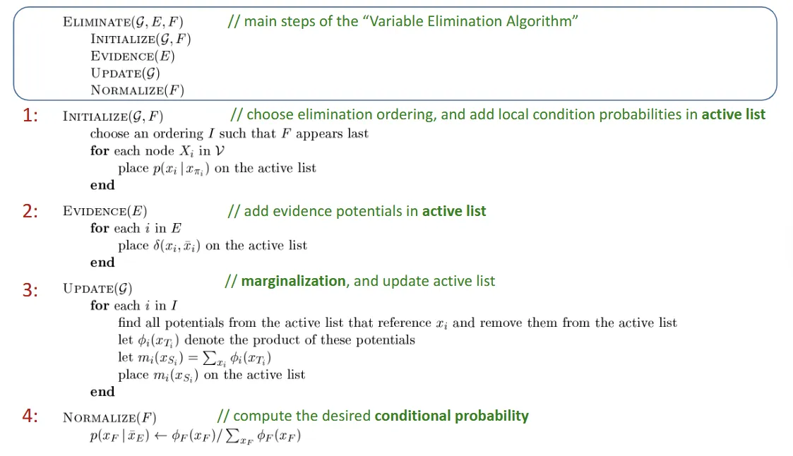
Variable elimination algorithm for Undirected Graph#

• Only change in initialize step
  • local condition (parent-child relation from DGM) $\rightarrow$ potential of $𝜓_{x_c} (x_c)$
• e.g $p(x_1, \bar x_6) = \frac {1}{Z} \sum_{x_2}\sum_{x_3}\sum_{x_4}\sum_{x_5} 𝜓(x_1, x_2) 𝜓(x_1, x_3) 𝜓(x_2, x_4) 𝜓(x_3, x_5) 𝜓(x_2, x_5, x_6) 𝜓(x_6, \bar x_6)$

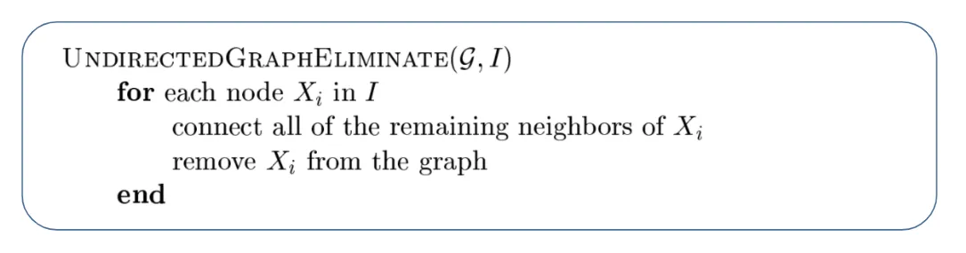
Reconstituted graph#

• Eliminate nodes and connect its (remaining) neighbors following the elimination order
• Reconstituted graph: original graph + new added edges
• complexity: the size of the largest clique in reconstructed graph
• Treewidth: smallest overall complexity $-1$ (NP-hard)
  • we want to minimize the cardinality of largest elimination clique

Moralization#

to trandorm DGM to UGM

• for every node in DGM, link its parents together to trandform to UGM
• So, to transfrom DGM to reconstituted graph DIRECTEDGRAPHELIMINATE
  • first we moraliza the DGM,
  • then we perform the UNDIRECTEDGRAPHELIMINATE algorithm

WARNING

We need to re-run for every query node to get each singleton conditional probability! Very inefficient!

• Sol: use the sum-product algorithm to get all single-node marginals for tree-like structures

Tree-like structures#

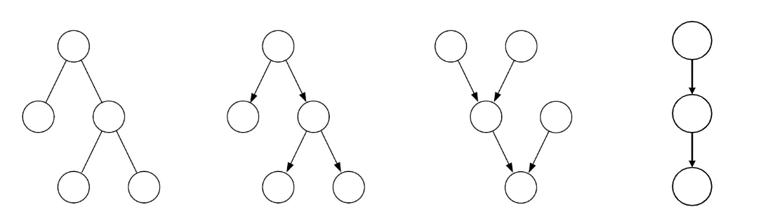
• (a) Undirected tree: no loop
• (b) Directed tree: 1 single parent per node, moralizations will not add link
• (c) Polytree: nodes with more than 1 parent, moralization will lead to loops $\Rightarrow$ cannot perform sum-product algorithm
• (d) Chain: just another directed tree

Parameterization#

• Undirected tree: only single & pair in cliques
  • $p(x) = \frac {1}{Z} (\prod_{i \in V} 𝜓(x_i) \prod_{(i, j) \in \epsilon} 𝜓(x_i, x_j))$
• Directed tree: simply parent-child relationship
  • $p(x) = p(x_r) \prod_{(i, j) \in \epsilon} p(x_j|x_i)$
    • $p(x_r)$ is the root node
• THey are formally identical

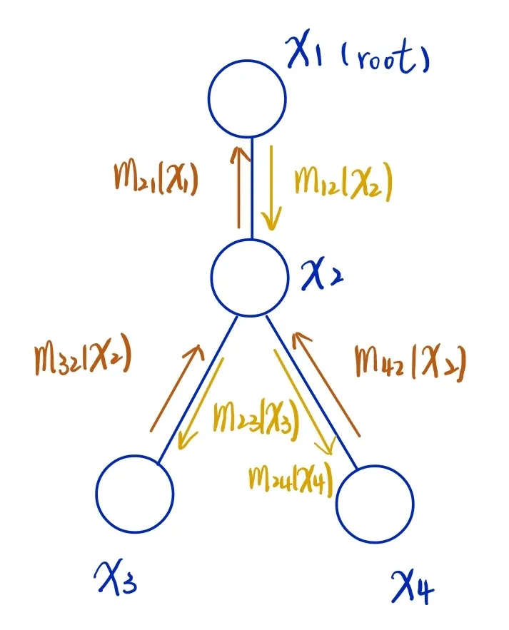
Message-Passing Protocol#

• a node can send a message to a neighbor only when it has received messages from all of its other neighbors (subtree), to ensure the messages passed to uppder node is complete.

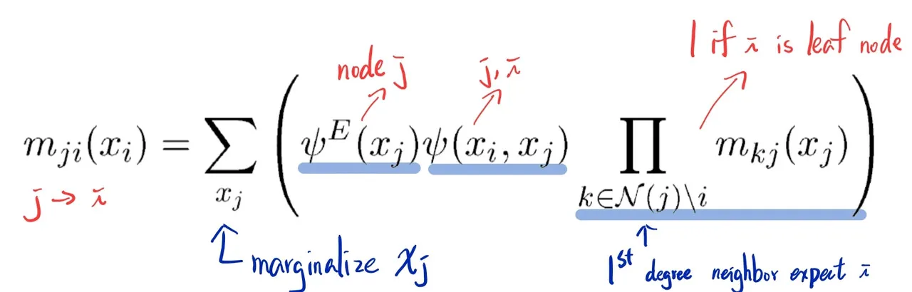
Message#

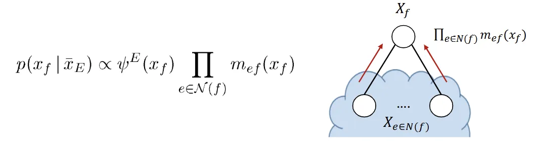
Compute marinal probability#

Sum-Product Algorithm a.k.a Belief Propogation#

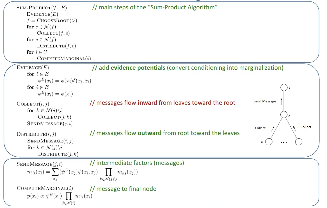
1. message flow from leaves to root (inward)
2. message flow from root to leaves (outward)